
How to Return the Second to Last Item in a List in Excel
- Drew Koontz
- May 29, 2023
- 2 min read
Usually, you need to return the last or first item in a list, but every once in a while, you may find yourself needing to return the second to last item in a list. These formulas will help.
Contents:
Formulas
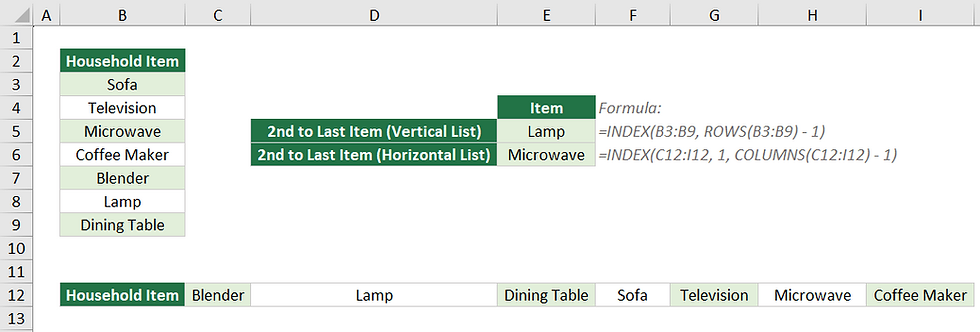
For both of these formulas, the "range" should be replaced with the vertical or horizontal list that you want to evaluate. For example, for a 100 item list in column A, you could use "A1:A100" for your range.
Formula to Return the Second to Last item in a Vertical List:
= INDEX(range, ROWS(range) - 1)Formula to Return the Second to Last item in a Horizontal List:
= INDEX(range, 1, COLUMNS(range) - 1)Examples
How to Return the 2nd to Last Non-blank Item in a Column
If we have a list of items in the range B3:B9, we can use the following formula to return the 2nd to last item from that list. The only thing that would need to be changed is the range you're evaluating.
It is important to note that this formula will ignore all blanks, only returning the last non-blank item.
= INDEX(B3:B9, ROWS(B3:B9) - 1)
How to Return the 2nd to Last Non-blank Item in a Row
We can use a similar formula if we have a horizontal list. The following formula will return the 2nd to last item from a row. The only thing that would need to be changed is the range you're evaluating.
It is important to note that this formula will ignore all blanks, only returning the last non-blank item.
= INDEX(C5:I5, 1, COLUMNS(C5:I5) - 1)


Comments